Global Path Planning and Local Path Planning for Mobile Robots
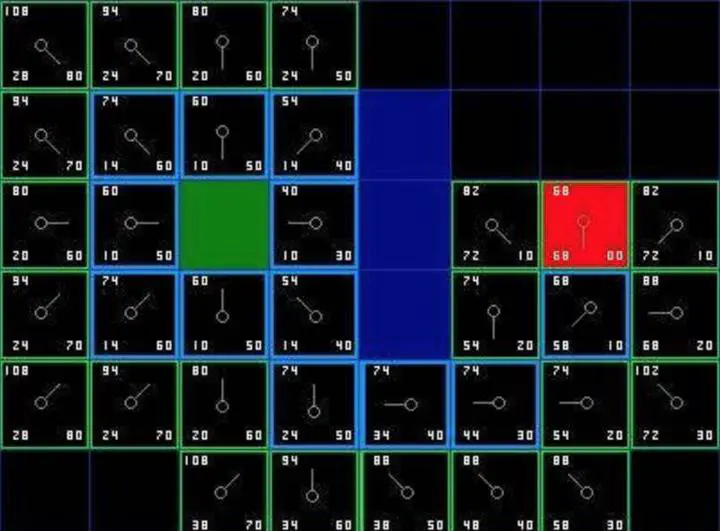 Photo by Zhang Tong on Unsplash
1 Global Path Planning
The A * algorithm is one of the most effective algorithms for global path planning methods in static environments. It not only considers the shortest distance from the extension point to the starting point, but also takes the shortest distance from the target point as a reference, which can not only achieve the shortest path, but also ensure the inspiration of the path points to avoid blind point selection. When there are few obstacles, fast planning can be carried out by changing the search neighborhood range, which can speed up the approximation to the target point. Its evaluation function is:
$$ F(n)=G(n)+F(n) $$
Where F (n) is the estimated value of the sum of the distance from node n to the starting point and the distance to the target point; G (n) is the estimated value of the distance from node n to the starting point; H (n) is the estimated value of the distance from node n to the target node. The point with the smallest estimated value F (n) is used as an alternative path node.
The workspace of the mobile robot is divided into two-dimensional raster map, which should contain the starting point, target point and surrounding obstacles information of the mobile robot. Usually, the starting point and the target point occupy only one grid, and the mobile robot is regarded as a particle point. The mobile robot searches for eight adjacent grids at a time, and selects the grid with the smallest cost value as an alternative extension point by calculating the cost estimate of the adjacent eight grids.
First, the following assumptions are made:
- The coordinates of the scalable node in the grid map are (xi, yi);
- The position of the target point is (xend, yend);
- H (xi, yi) is the estimated value of the heuristic distance, from which the distance between the two points can be estimated as:
Euclidean distance: The linear distance estimation method between two points is defined as:
$$ H(x_i,y_i)=\sqrt{(x_end-x_i)^2+(y_end-y_i)^2} $$
Manhattan distance: The Manhattan distance is composed of the sum of two distances, namely the horizontal distance and the vertical distance. Its expression can be defined as:
$$H(x_i,y_i)=abs(x_\text{end}-x_i)+abs(y_\text{end}-y_i)$$
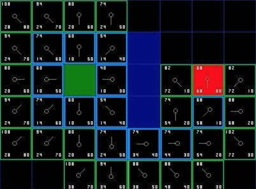
Each square in the figure is marked with the values of F, G, and H. The upper left corner is F, the lower left corner is G, and the lower right corner is H, where the green point is the starting point, the red point is the target point, the blue grid is the obstacle point, and the blue border grid forms a path from the starting point to the target point.
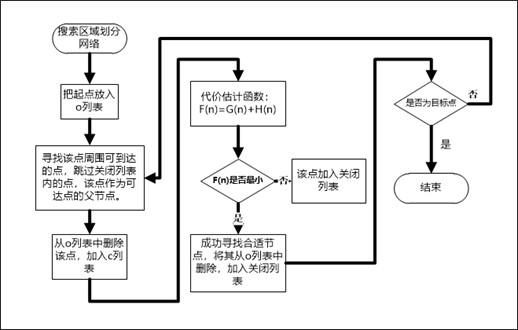
The A * algorithm usually creates two tables in the extended search, namely the open list and the closed list, hereinafter referred to as the “O table” and the “C table” respectively. The trajectory of the optimal path planned in the future is the trajectory composed of the points stored in the O table. The expansion steps are:
1.After completing the division of the area, set the starting point to the current point, that is, (S) into the O table, and clear the C table to zero;
2.Put the expandable points n around S (the grid occupied by the obstacle is a non-expandable point) into the O table, and the starting point S is the parent node;
3.Retrieve whether there is an expandable point in the O list, if not, the pathfinding fails; if there is, continue the search;
4.Put the current point into table C, and calculate the cost value F of the scalable point n in table O through the cost function, and set the point with the smallest F value as the current point, and at the same time as the parent node, put other scalable points into table C;
5.Put the expandable nodes around the current point into the O table, and determine whether the current point is the target node. If so, end the entry. 6.All the parent nodes in the algorithm process are traced back, which is the shortest path.
The flow chart of the A * algorithm can be expressed as follows:
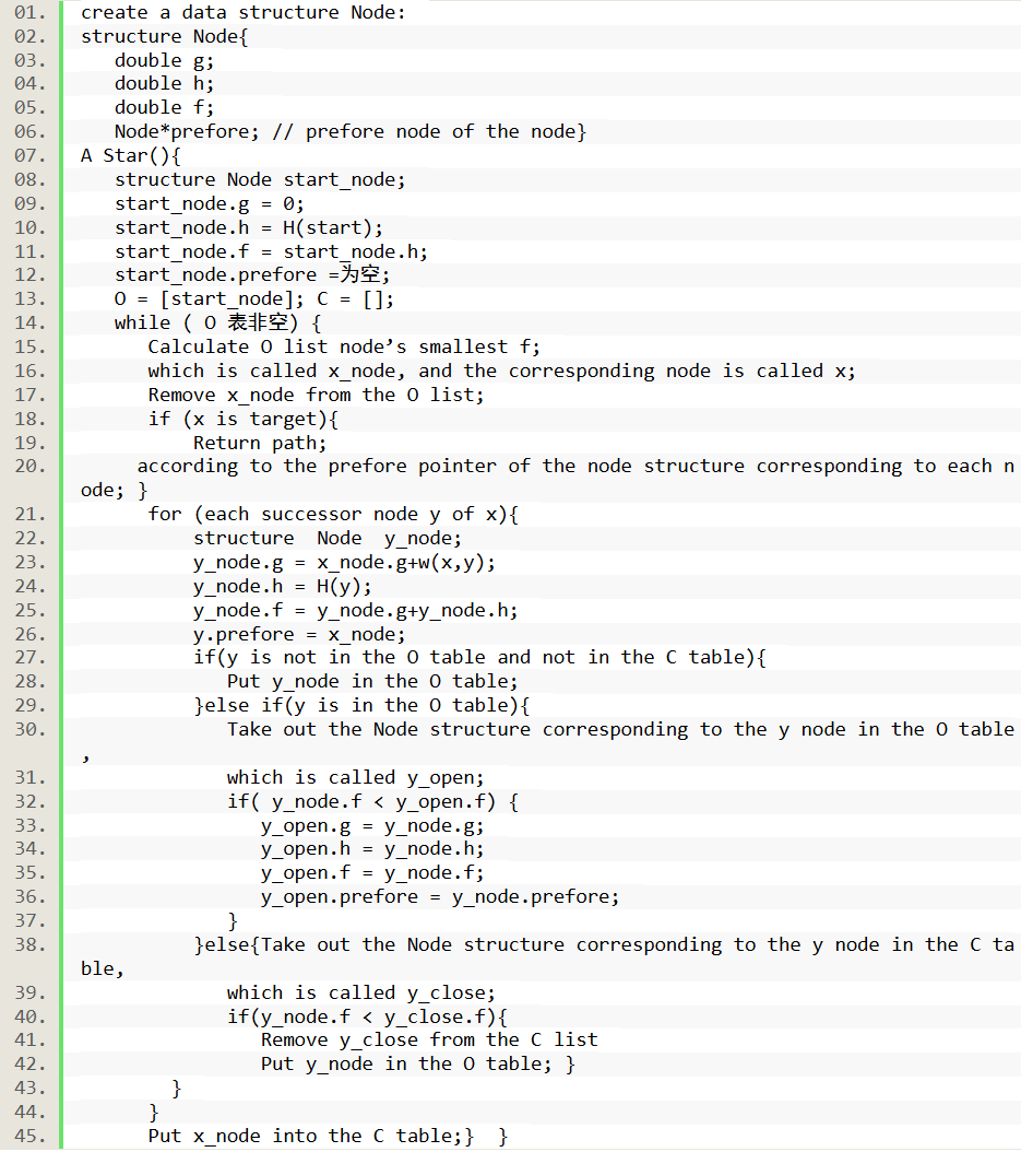
The experimental program design pseudocode based on the A * algorithm is as follows: create a data structure Node:
MATLAB R2016a is used to experiment with the algorithm. The size of the environment map is 40 * 80 rectangular grid map as shown in the figure. The construction of the environment simulates the warehousing and logistics scene, which includes six rows of neatly arranged shelves. The obstacles marked at the four corners are simulated building structures. Other random obstacles that may exist in this paper are not set, such as other robots at work.
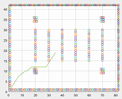
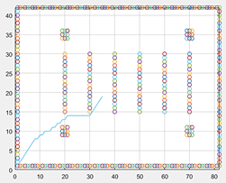
From the graph, two methods of distance prediction function can be known: (a) A * algorithm path based on Euclidean distance prediction to target point distance estimate; (b) A * path graph based on Manhattan distance prediction to target point distance estimate.
2 Local Path Planning
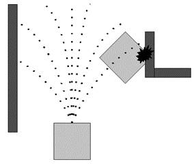
The Dynamic Window Approach (DWA) algorithm restricts the traditional mobile robot to the method of using position control to achieve obstacle avoidance, and converts the cohesion into the method of using the speed prediction control of the mobile robot in the next cycle to achieve obstacle avoidance. Therefore, the window of the dynamic window is the speed window [8]. The dynamic window refers to simulating a series of speeds of the mobile robot’s forward direction at the next moment to form a two-dimensional speed space (including linear velocity and angular velocity). Predicting the path of the alternative speed space eliminates the speed that may collide with the obstacles in the environment, and then selects an optimal speed from the feasible speed space as the speed of the next motion cycle, as shown in the figure.
(1) Kinematic modeling of mobile robots based on DWA algorithm
The predicted trajectory set of the mobile robot can be used to form a series of arcs and curves in the forward direction of the robot. As shown in Figure 4.5, because the mobile robot can move a limited distance in one cycle, its trajectory can be approximated as a straight line. That is, in the robot coordinate system, the distance of the axis movement is V_t\ times\ mathrm {\ Delta t}, and the projected distance in the x-axis and y-axis directions of the world coordinate system is calculated respectively. That is, the distance delta x and delta y traveled by the mobile robot in the world coordinate system in one delta t cycle can be obtained, which are expressed as:
$$I\left{\begin{matrix}\Delta x=V_t\times\Delta t\times\cos\theta_t\\Delta y=V_t\times\Delta t\times\sin\theta_t\end{matrix}\right.$$
Thus the motion model of the mobile robot after one cycle of operation is:
$$\begin{cases}x=x+V_t\times\Delta t cos(\theta_t)=x+V_x\times\Delta t cos(\theta_t)-V_y\times\Delta t sin(\theta_t)\y=y+V_t\times\Delta t sin(\theta_t)=y+V_x\times\Delta t cos(\theta_t)+V_y\times\Delta t sin(\theta_t)\\theta_t=\theta_t+w_t\Delta t\end{cases}$$
x, y is the horizontal axis coordinates and vertical axis coordinates of the current position of the mobile robot in the world coordinate system; V_t is the speed of the mobile robot at time t; V_x, V_y is the speed in the x-axis and y-axis directions in the world coordinate system;\ theta_t is the angle between the robot and the world coordinate system x-axis at time t; w_t is the angular velocity of the mobile robot at time t.
(2) velocity space constraint
1.Based on kinematic velocity constraint
In the speed space, the mobile robot is first affected by the hardware device, and the most intuitive is limited by the motor speed. Therefore, the speed space of the mobile robot needs to meet the basic kinematic constraints:
$$V_{s}={v\in[vmax_{min},w\in[wmax_{min}]]}$$
V_s is the size of the speed space obtained by the motor performance; v_ {min} is the minimum speed that the mobile robot can achieve by the motor; v_ {max} is the maximum speed that the mobile robot can achieve by the motor performance; w_ {min}, w_ {max} is the minimum angular velocity and maximum angular velocity that the mobile robot can achieve by the motor performance.
2.Based on Dynamic Velocity Constraint
The maximum acceleration that a mobile robot can achieve also places a limit on the speed, so the robot can actually reach a speed of:
$$V_d={(v,w)\mid v\in[v_{\mathrm{now}}-\dot{v}b\Delta t,v{\mathrm{now}}+\dot{v}a\Delta t]\cap w\in[w{\mathrm{now}}-\dot{w}b\Delta t,w{\mathrm{now}}+\dot{w}_a\Delta t]}$$
where is the size of the velocity space affected by acceleration; and are the linear and angular velocities of the mobile robot at the current moment; {\dot{v}}_a and {\dot{w}}_a are the maximal linear and maximal angular accelerations of the mobile robot; and {\dot{v}}_b and {\dot{w}}_b are the maximal linear deceleration and maximal angular deceleration;
3.Speed constraints based on safe distances from obstacles
Ensure that the mobile robot can be stopped at a safe distance with maximum deceleration.
$$V_{a}=\left{(v,w)\mid v\leq\sqrt{2\times dist(v,w)\times\dot{v}{b}}\cap w\leq\sqrt{2\times dist(v,w)\times\dot{w}{b}}\right}$$
Where V_a is the feasible velocity space under the condition of ensuring a safe distance without collision; dist(v,w) is the minimum safe distance of the mobile robot from the obstacle;
The feasible velocity space established by the dynamic window is the velocity space provided by the intersection of the above three, three constrained velocity spaces, viz:
$$V_{robot}=V_S+V_d+V_a$$
The DWA algorithm is widely used for its simple model and intuitive use of variables that do not require further complex derivations. The mathematical model of the DWA algorithm is established for the alternative velocity space formed by the mobile robot, which is referred to as the evaluation function in the paper, and the optimal combination of velocity and angular velocity is selected through the evaluation function. Where the evaluation function formula is:
$$G=\sigma(\alpha\times head (v,w)+\beta\times dist(v,w)+\gamma\times velocity (v,w))$$
Where \ head\ (v,w) is the direction angle scoring function; dist(v,w) is the distance scoring function between the robot and the obstacle; \ velocity\ (v,w) is the velocity scoring function of the mobile robot; is the weight factor of the heading angle scoring function; is the weight factor of the distance scoring function with the obstacle; is the weight factor of the velocity scoring function.
The direction of motion of the mobile robot is determined by the magnitude of the evaluation function’s G. The larger the value of G, the greater the likelihood that the direction of the trajectory formed by the combination of that velocity and the angular velocity will be used as the direction of the mobile robot at the next moment. Three weighting factors in the mathematical model Used to regulate the effect of different rating functions on the mathematical model.
The magnitude of the predicted speed of the mobile robot is used as the score, and the greater the speed of the mobile robot is expected to be, the better it is when it is guaranteed to be safe and close to the target point. The processing formula for normalising the scoring function is as follows:
$$head_{normal}\left(i\right)=\frac{head\left(i\right)}{\sum_{i=1}^{n}head\left(i\right)}$$ $$dist_{normal}(i)=\frac{dist(i)}{\sum_{i=1}^{n}dist(i)}$$ $$velocity_{normal}\left(i\right)=\frac{velocity(i)}{\sum_{i=1}^{n}velocity(i)}$$
Where:n denotes the number of all current trajectories sampled; i denotes the ith sampled trajectory; \ head(i), dist(i), velocity(i) are the direction angle score, obstacle closest distance score, and velocity score of the ith trajectory, respectively; \ head_{normal}(i), distnormal(i), velocitynormal(i) are the direction angle score, obstacle nearest distance score, and velocity score normalisation results for the ith trajectory, respectively.
By scoring and filtering the predicted trajectories of the mobile robot simulation, the trajectories that are predicted to have the potential to hit obstacles are removed from the set of speeds, and from the remaining feasible speeds, the combination of speeds and linear velocities with the largest scores of the evaluation function is selected, and this combination is used as the trajectory for the mobile robot travelling in the next cycle.
Based on the MATLAB R2016a simulation, a raster map with different numbers of obstacles is established for simulation planning, and in this experiment, the mobile robot is set to have a starting point at (0,0) and a target point at (7,6). The experiment makes the following parameter settings: the maximum speed of the mobile robot is 1m/s; the maximum angular velocity is 2rad/s; the maximum linear acceleration is 3m/s2; the maximum rotational acceleration is set to 4rad/s2; the resolution of speed is 5m/s; the resolution of angular velocity is 6rad/s; the resolution of time is 0.1s; and the simulation time of the forward simulation track is 4s. Simulation study of the original DWA algorithm: mobile robots working in the same environmental state using a fixed combination of parameters, the effect is shown in the figure.
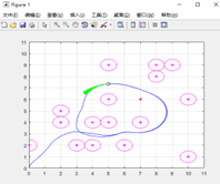
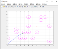
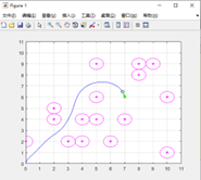
The experimental simulation results are shown in Fig. (a) The combination of weights is , the robot can smoothly pass through the obstacles in the dense area, which indicates that the mobile robot has the ability of obstacle avoidance and exploration and has the tendency to approach to the target point (7,6) after circling around the obstacles, but it does not arrive at the target point, and it is stuck in a loop. In the DWA algorithm, the weights are used to determine the magnitude of the tendency to steer the robot towards the target point. The reason for not reaching the target point is that the weights of the direction angle scoring function are not sufficiently enlightening for the target point with low weights. As shown in figure (b) the combination of weights is , the mobile robot is guided in a direction that is always towards the target point, but when travelling to position (3.5,3.5) it is blocked by an obstacle and the mobile robot is not able to enter the obstacle zone. The experiments illustrate that the mobile robot direction angle scoring function weights are larger, the robot’s exploration performance decreases the problem of goal unreachability. As shown in Fig. (c) the weight combination is , the mobile robot successfully reaches the target point with a more reasonable trajectory.
张通
Student of Mechatronic Engineering
My research interests include control system, robotics technology and micromanipulation.